set.seed(17)
n_blank <- 60                      # assumption, not a quoted requirement
blank <- rnorm(n_blank, mean = 0.5, sd = 0.40)        # pg/mL
low_lv <- c(1.0, 1.5, 2.0, 2.5, 3.0); reps <- 12
low <- data.frame(level = rep(low_lv, each = reps))
low$y <- rnorm(nrow(low), low$level, 0.45)3. Detection capability (EP17) and linearity (EP06)
Tags: [S] primary public source, [Y] my synthesis. All data below are simulated.
(a) Concept
| Term | Question it answers | Typical statement |
|---|---|---|
| LoB | Highest result expected from a blank | 95th percentile of blank results |
| LoD | Lowest concentration reliably distinguished from the LoB | ≥95% of results above the LoB |
| LoQ | Lowest concentration measured with acceptable error (CV or total-error goal) | CV ≤ goal, or bias + 1.96·SD ≤ allowable error |
| Linearity | Does response scale proportionally with concentration across the range? | polynomial vs linear fit; allowable deviation |
Two error types fix LoB and LoD: α = 5% false positive (blank above LoB), β = 5% false negative (low sample below LoB). [Y]
(b) Regulatory anchor
| Item | Fact | Tag |
|---|---|---|
| EP17 | EP17-A2 (2012, confirmed 2017); no newer edition listed. Evaluates and verifies LoB, LoD, LoQ claims | [S] clsi.org |
| EP06 | Ed2 (2020-11-24): low-cost linearity validation incl. LLoQ/ULoQ; two designs (high sample + measurand-free, or high and low samples) | [S] clsi.org |
| IVDR | Annex I 9.1(a) lists “limits of detection and quantitation, measuring range, linearity” | [S] |
| Design counts (EP17: blanks, lots, days; EP06 replicates) | not verified: paywalled. Simulation sizes below are my assumptions | – |
(c) R lab
Simulated study
LoB and LoD, parametric and nonparametric
lob_p  <- lob_param(blank)
lob_np <- lob_nonparam(blank)
# pooled within-level SD of low samples
sd_low <- sqrt(mean(tapply(low$y, low$level, var)))
lod_p_check <- lob_p + 1.645 * sd_low
sd_low_lm <- sigma(lm(y ~ factor(level), low))        # pooled SD from an ANOVA fit

# Nonparametric LoD: lowest level whose results are >= 95% above the LoB
hit <- tapply(low$y > lob_np, low$level, mean)
lod_np <- as.numeric(names(hit)[which(hit >= 0.95)[1]])

kable(data.frame(
  Quantity = c("LoB", "LoD"),
  Parametric = round(c(lob_p, lod_p_check), 3),
  Nonparametric = round(c(lob_np, lod_np), 3),
  Formula = c("mean + 1.645·SD_blank", "LoB + 1.645·SD_low (pooled)")),
caption = "Detection capability (pg/mL)")| Quantity | Parametric | Nonparametric | Formula |
|---|---|---|---|
| LoB | 1.251 | 1.254 | mean + 1.645·SD_blank |
| LoD | 2.040 | 2.500 | LoB + 1.645·SD_low (pooled) |
kable(data.frame(level = names(hit), `fraction above LoB (np)` = round(as.numeric(hit), 3),
check.names = FALSE), caption = "Hit rate of low-level samples")| level | fraction above LoB (np) |
|---|---|
| 1 | 0.167 |
| 1.5 | 0.583 |
| 2 | 0.917 |
| 2.5 | 1.000 |
| 3 | 1.000 |
stopifnot(isTRUE(all.equal(sd_low, sd_low_lm))) # hand pooled SD = lm sigmaPlain 1.645 multipliers are the textbook parametric formulas; small-sample correction factors in EP17 are not verified: paywalled. [Y]
Cross-check of the parametric LoB by simulation
# Under normality the 95th percentile of the blank distribution is mean + 1.645 sd.
big <- rnorm(1e6, 0.5, 0.40)
c(theory = 0.5 + 1.645 * 0.40, big_sim_q95 = unname(quantile(big, .95)),
  estimate_from_n60 = lob_p)
theory big_sim_q95 estimate_from_n60
1.158000 1.157291 1.250696 Probit LoD (hit-rate design, molecular assays) [Y]
conc <- c(2, 4, 7, 10, 15, 25, 50); n <- rep(24, length(conc))
b1 <- 2.5; b0 <- qnorm(.95) - b1 * log10(10)              # true LoD95 = 10
hits <- rbinom(length(conc), n, pnorm(b0 + b1 * log10(conc)))
fit <- glm(cbind(hits, n - hits) ~ log10(conc), family = binomial("probit"))
dp <- dose.p(fit, p = 0.95)
lod_dose <- 10^as.numeric(dp)
lod_hand <- lod_probit(conc, hits, n)
ci_log <- as.numeric(dp) + c(-1, 1) * 1.96 * attr(dp, "SE")
kable(data.frame(method = c("MASS::dose.p", "hand inversion"),
LoD95 = round(c(lod_dose, lod_hand), 2)))| method | LoD95 |
|---|---|
| MASS::dose.p | 7.15 |
| hand inversion | 7.15 |
cat(sprintf("Delta-method 95%% CI: %.1f - %.1f copies/mL (true value 10)\n",
            10^ci_log[1], 10^ci_log[2]))
Delta-method 95% CI: 5.3 - 9.7 copies/mL (true value 10)stopifnot(isTRUE(all.equal(lod_dose, lod_hand)))This is one realisation; a single 95% CI misses the truth about 1 time in 20. Coverage check over 1000 repeats of the same design:
set.seed(2024)
cover <- replicate(1000, {
  h <- rbinom(length(conc), n, pnorm(b0 + b1 * log10(conc)))
  f <- suppressWarnings(glm(cbind(h, n - h) ~ log10(conc), family = binomial("probit")))
  d <- suppressWarnings(dose.p(f, p = 0.95))
  r <- as.numeric(d) + c(-1, 1) * 1.96 * attr(d, "SE")
  1 >= r[1] && 1 <= r[2]       # log10(10) = 1
})
c(coverage = mean(cover))
coverage
0.937 Parametric bootstrap of the LoD (my method)
Resample blank and low-level results from the fitted normals, recompute LoD, take percentiles.
set.seed(99)
B <- 4000
lod_b <- replicate(B, {
  b <- rnorm(n_blank, mean(blank), sd(blank))
  l <- rnorm(length(low_lv) * reps, 0, sd_low)          # centred; only the SD enters
  lob_param(b) + 1.645 * sd(l)
})
# Cross-check against the exact chi-square distribution of the pooled SD part:
# Var(SD_low*) approx; compare the bootstrap SE with the delta-method SE.
se_delta <- sqrt(sd(blank)^2 / n_blank +
  1.645^2 * sd(blank)^2 / (2 * (n_blank - 1)) +
  1.645^2 * sd_low^2 / (2 * length(low_lv) * (reps - 1)))
c(LoD_point = lod_p_check, boot_median = median(lod_b),
  boot_CI_lo = unname(quantile(lod_b, .025)), boot_CI_hi = unname(quantile(lod_b, .975)),
  boot_SE = sd(lod_b), delta_SE = se_delta)
LoD_point boot_median boot_CI_lo boot_CI_hi boot_SE delta_SE
2.0396742 2.0359937 1.8172921 2.2430930 0.1092108 0.1124553 How to defend each (one paragraph). Parametric uses all observations and gives a smooth estimate with a CI, but rests on normality of blank and low-level results; check with a QQ-plot and consider a log scale if blanks are skewed. Nonparametric assumes nothing about the shape but is a coarse rank statistic: with 60 blanks the 95th percentile is determined by about three values and with 12 replicates per level the hit rate can only change in steps of 8%. Probit is the right tool when the outcome is hit/no-hit, as in qPCR. Parametric bootstrap is my uncertainty statement on the parametric LoD: it adds a CI and exposes how few df the SD of the low samples really has; it inherits the normality assumption and is not a CLSI-prescribed procedure. [Y]
LoQ from a precision profile
set.seed(5)
lv <- c(1, 2, 3, 5, 8, 12, 20); r <- 20
sd_true <- function(c) sqrt(0.30^2 + (0.06 * c)^2)
pp <- data.frame(level = rep(lv, each = r))
pp$y <- 1.03 * pp$level + rnorm(nrow(pp), 0, sd_true(pp$level))   # +3% proportional bias
s <- aggregate(y ~ level, pp, function(v) c(m = mean(v), s = sd(v)))
s <- data.frame(level = s$level, mean = s$y[, "m"], sd = s$y[, "s"])
s$cv <- 100 * s$sd / s$mean
s$total_error_pct <- 100 * (abs(s$mean - s$level) + 1.96 * s$sd) / s$level
kable(s, digits = 2, caption = "Precision profile; CV goal 20%, total-error goal 30% (assumed goals)")| level | mean | sd | cv | total_error_pct |
|---|---|---|---|---|
| 1 | 0.94 | 0.28 | 30.12 | 61.31 |
| 2 | 2.19 | 0.38 | 17.23 | 46.78 |
| 3 | 3.13 | 0.29 | 9.41 | 23.65 |
| 5 | 5.05 | 0.31 | 6.16 | 13.29 |
| 8 | 8.31 | 0.52 | 6.20 | 16.53 |
| 12 | 12.39 | 0.95 | 7.66 | 18.76 |
| 20 | 20.47 | 1.36 | 6.65 | 15.67 |
loq_cv <- s$level[which(s$cv <= 20)[1]]
loq_te <- s$level[which(s$total_error_pct <= 30)[1]]
# model-based: sd^2 = a^2 + b^2 c^2 by weighted lm on variances
m <- lm(I(sd^2) ~ 1 + I(level^2), s)
a2 <- coef(m)[1]; b2 <- coef(m)[2]
loq_model <- sqrt(a2 / (0.04 - b2))
c(LoQ_empirical_CV20 = loq_cv, LoQ_empirical_TE30 = loq_te, LoQ_model_CV20 = unname(loq_model))
LoQ_empirical_CV20 LoQ_empirical_TE30 LoQ_model_CV20
2.000000 3.000000 1.375589 Linearity (EP06 style, polynomial comparison) [Y]
set.seed(8)
x <- rep(seq(0, 100, length.out = 9), each = 2)
mu <- 20 + x - 0.0018 * x^2                 # mild saturation
y <- mu + rnorm(length(x), 0, 0.01 * mu)
chk <- linearity_check(x, y, degree = 3)
# hand F-test
lin <- lm(y ~ x); cub <- lm(y ~ poly(x, 3, raw = TRUE))
F_hand <- ((deviance(lin) - deviance(cub)) / 2) / (deviance(cub) / df.residual(cub))
c(F_function = chk$F, F_hand = F_hand, p = chk$p_nonlinear)
F_function F_hand p
3.502025e+01 3.502025e+01 3.560210e-06 stopifnot(isTRUE(all.equal(chk$F, F_hand)))
kable(data.frame(level = names(chk$deviation_pct), deviation_pct = round(chk$deviation_pct, 2),
within_5pct = abs(chk$deviation_pct) <= 5),
caption = "Deviation of linear from cubic fit (allowable ±5%, assumed goal)")| level | deviation_pct | within_5pct | |
|---|---|---|---|
| 0 | 0 | 11.54 | FALSE |
| 12.5 | 12.5 | 1.33 | TRUE |
| 25 | 25 | -1.81 | TRUE |
| 37.5 | 37.5 | -2.59 | TRUE |
| 50 | 50 | -2.33 | TRUE |
| 62.5 | 62.5 | -1.54 | TRUE |
| 75 | 75 | -0.50 | TRUE |
| 87.5 | 87.5 | 0.67 | TRUE |
| 100 | 100 | 1.87 | TRUE |
df <- data.frame(x, y)
ggplot(df, aes(x, y)) + geom_point() +
  geom_smooth(method = "lm", se = FALSE, colour = "grey40", linetype = 2) +
  geom_smooth(method = "lm", formula = y ~ poly(x, 3), se = FALSE, colour = "#d95f02") +
  labs(x = "Expected concentration", y = "Measured") + theme_minimal()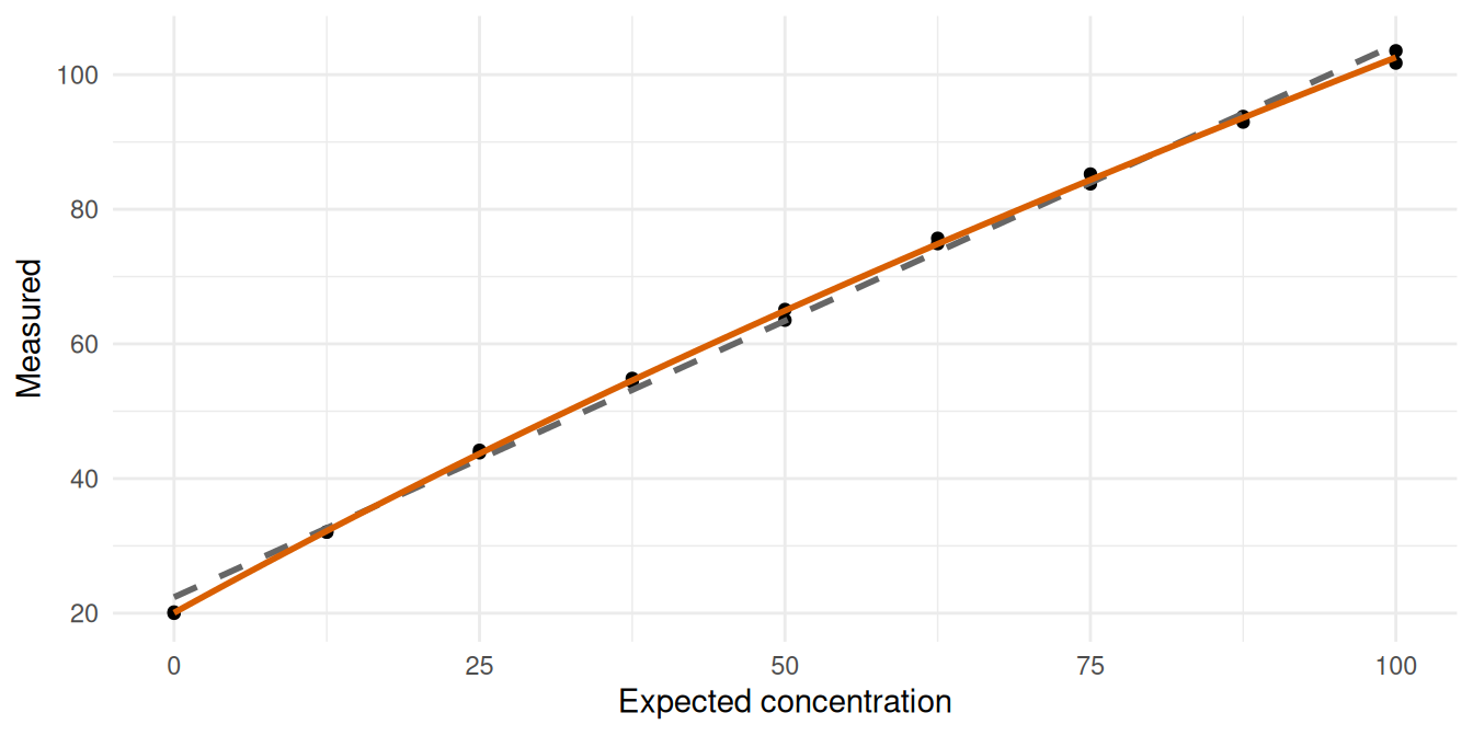
The F-test shows real curvature, but the decision uses the deviation limit: here only the lowest level exceeds ±5% (the straight line overshoots at the low end), so a defensible claim restricts the linear range to start above it and re-tests. A significant F-test alone is not a failure, and a non-significant one is not proof of linearity in a small study. [Y]
(d) Claims
EP17-A2, EP06-Ed2 editions and scope, IVDR Annex I 9.1(a) are in the ledger. Design counts for EP17 and EP06: not verified: paywalled.