6. Cut-offs, two-cut-off designs and the intermediate zone
Tags: [S] primary public source, [Y] my synthesis, [D] derived by me by arithmetic from a cited count. The lab uses simulated data only.
(a) Concept
Idea
Meaning
Single cut-off
one threshold; Youden (max Se+Sp−1), a targeted Se or Sp, or cost-weighted
Two cut-offs
rule-out cut-off set for sensitivity/NPV; rule-in cut-off set for specificity/PPV
Intermediate (“grey”) zone
results between the two; the price paid for high predictive values
Lock before validation
derive on one cohort, freeze, validate on another; never re-tune on validation data
Spectrum and prevalence
the same cut-offs give different zone fractions and PPV/NPV in primary vs specialty care
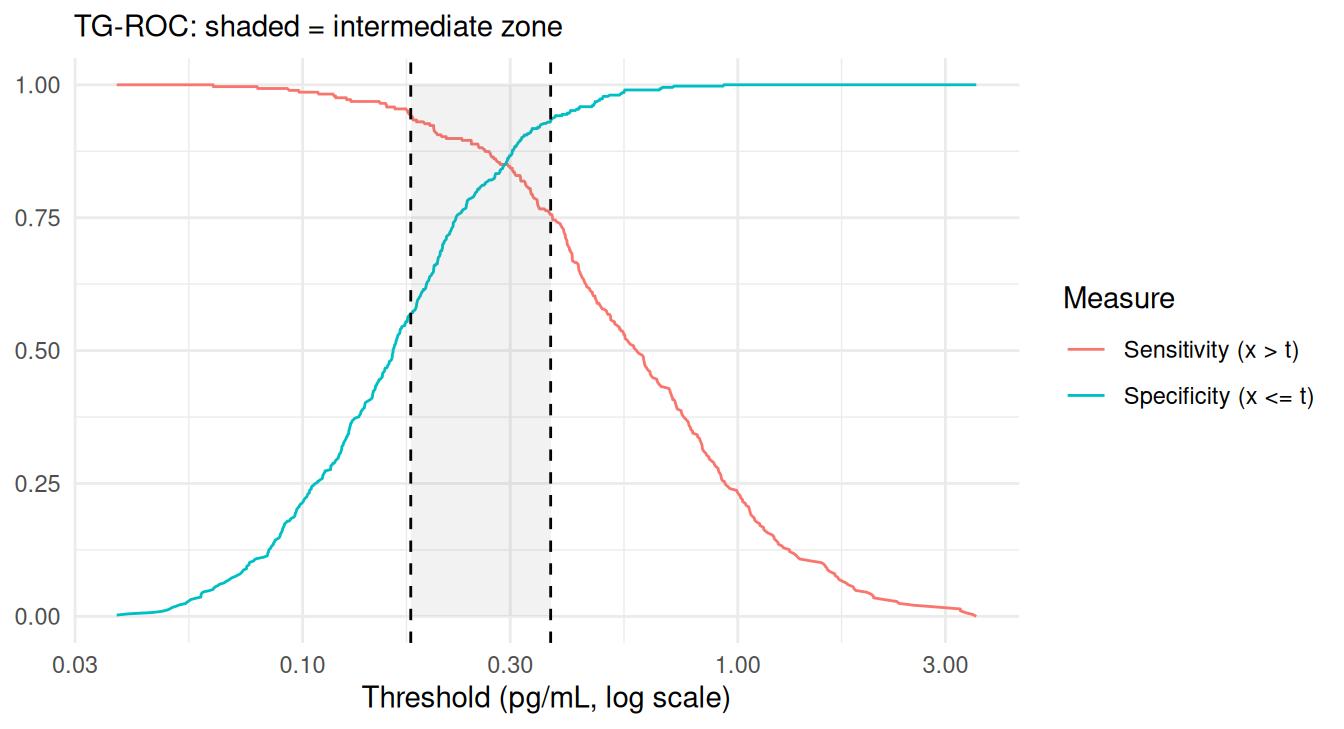
Grey-zone approach: Coste & Pouchot, Int J Epidemiol 2003;32:304-313 [S: abstract]: a three-zone partition whose width depends on the separation of the group means, variability, and the accepted misclassification risks. TG-ROC plots sensitivity and specificity against the threshold so the zone limits can be read off.
(b) Regulatory anchor and worked example: Elecsys Phospho-Tau (217P) Plasma
Facts below were read from the FDA 510(k) Decision Summary K261686 (37 pp.) and re-checked by me against the PDF for the tables marked ✔. Everything else is from the research notes (research/ptau217_notes.md).
Item
Value
Source
510(k) / decision
K261686, decision 2026-08-19, SESE, Class II, 21 CFR 866.5840 “Alzheimer’s Disease Pathology Assessment Test”
FDA-DS p.1, openFDA record
Predicate
Lumipulse G pTau 217/beta-Amyloid 1-42 Plasma Ratio, K242706 ✔
FDA-DS p.4
Indication
aid in identifying amyloid pathology in patients with cognitive decline, plasma of individuals ≥ 55 years, used with other clinical information ✔
Reproduce what FDA reported, then compare our CI methods with theirs:
N <-sum(fda); pet_pos <-sum(fda[, 1]); pet_neg <-sum(fda[, 2])rows <-list(c("PPA (positive among PET+)", 285, pet_pos, "75.4 (70.8-79.5)"),c("NPA (negative among PET-)", 424, pet_neg, "73.1 (69.4-76.6)"),c("PPV of positive", 285, 322, "88.5 (84.9-91.4)"),c("NPV of negative", 424, 445, "95.3 (93.1-96.8)"))out <-do.call(rbind, lapply(rows, function(r) { x <-as.numeric(r[2]); n <-as.numeric(r[3]); w <-ci_wilson(x, n); cp <-ci_clopper_pearson(x, n)data.frame(Measure = r[1], `FDA reported`= r[4],`Wilson`=sprintf("%.1f (%.1f-%.1f)", 100* w[1], 100* w[2], 100* w[3]),`Clopper-Pearson`=sprintf("%.1f (%.1f-%.1f)", 100* cp[1], 100* cp[2], 100* cp[3]),check.names =FALSE)}))kable(out, caption ="FDA CIs vs ours. FDA states the PV CIs derive from likelihood-ratio CIs; the PPA/NPA CI method is not stated")
FDA CIs vs ours. FDA states the PV CIs derive from likelihood-ratio CIs; the PPA/NPA CI method is not stated
Measure
FDA reported
Wilson
Clopper-Pearson
PPA (positive among PET+)
75.4 (70.8-79.5)
75.4 (70.8-79.5)
75.4 (70.7-79.7)
NPA (negative among PET-)
73.1 (69.4-76.6)
73.1 (69.4-76.6)
73.1 (69.3-76.7)
PPV of positive
88.5 (84.9-91.4)
88.5 (84.6-91.5)
88.5 (84.5-91.8)
NPV of negative
95.3 (93.1-96.8)
95.3 (92.9-96.9)
95.3 (92.9-97.1)
Our Wilson intervals reproduce FDA’s PPA and NPA CIs to the printed digit (70.8-79.5, 69.4-76.6), so Wilson is the likely method [D: inference, not stated by FDA]. The PV CIs differ slightly because FDA derives them from likelihood-ratio CIs.
The PPA/NPA are low (≈75%) because intermediates count as misses (denominators include all PET+ and PET−). The headline strength is in the categories: PV 88.5% for positive, 95.3% NPV for negative, 19.9% (191/958) intermediate ✔. Derived by me [D] from the counts above (no CI in the FDA summary):
Also FDA’s decision logic is worth noting: the PV is judged “statistically higher than prevalence” (lower CI bound 84.9% > prevalence 39.5%), a comparison with the prevalence rather than a pre-specified performance goal; none of a sample-size calculation or goal was found in the text read. ✔ (FDA-DS p.27)
Known blemishes in the summary (do not copy tables uncritically) ✔: p.26 says “pre-specified cut-offs of 0.225 pg/mL” while the table uses 0.223, and “prevalence 13.1%” in one sentence vs 39.5% elsewhere; others are listed in the notes.
What the two papers do and do not give. Both use the prototype assay, not the cleared one, and neither reports 0.223/0.378. Hibar et al., Alzheimers Dement 2026;22(1):e71009: five cohorts, N = 2,148, single rule-out cut-off 0.189 pg/mL, no intermediate zone; e.g. cognitively impaired (n = 538) sensitivity 98.98%, specificity 29.17%, NPV 92.51% [S]. Hortsch et al., J Prev Alzheimers Dis 2026;13(5):100534: APPROACH, N = 588, centiloid reference, exploratory double cut-off at 90% PPA / 90% NPA, indeterminate 5.78% at centiloid 30, Wilson CIs, eGFR distribution reported and “higher pTau217 with worse kidney function” [S]. Nothing here is the pivotal data behind the clearance.
(c) R lab (simulated)
Cohorts
pTau217-like: log10 concentration normal in both groups, higher in amyloid-positive.
Targets (assumed): sensitivity ≥ 94% for the rule-out step, specificity ≥ 93% for the rule-in step, chosen to resemble the derived operating points of the public pivotal data. [Y]
co <-derive_two_cutoffs(train$x, train$y, 0.94, 0.93)# cross-check 1: cutpointra <-cutpointr(train, x, y, pos_class =1, neg_class =0, direction =">=",method = maximize_metric, metric = spec_constrain, min_constrain =0.94)b <-cutpointr(train, x, y, pos_class =1, neg_class =0, direction =">=",method = maximize_metric, metric = sens_constrain, min_constrain =0.93)# cross-check 2: OptimalCutpointsoc_lo <-optimal.cutpoints(X ="x", status ="y", tag.healthy =0, methods ="ValueSe",control =control.cutpoints(valueSe =0.94), data = train)oc_hi <-optimal.cutpoints(X ="x", status ="y", tag.healthy =0, methods ="ValueSp",control =control.cutpoints(valueSp =0.93), data = train)pick <-function(o, nm) as.numeric(o$Global$optimal.cutoff[[nm]])[1]oc_lo_c <-pick(oc_lo$ValueSe, "cutoff"); oc_lo_se <-pick(oc_lo$ValueSe, "Se")oc_hi_c <-pick(oc_hi$ValueSp, "cutoff"); oc_hi_sp <-pick(oc_hi$ValueSp, "Sp")se_at <-function(c) mean(train$x[train$y ==1] > c)sp_at <-function(c) mean(train$x[train$y ==0] <= c)kable(data.frame(Method =c("hand", "cutpointr", "OptimalCutpoints"),`Rule-out cut-off`=round(c(co[["lo"]], a$optimal_cutpoint, oc_lo_c), 4),`Sens at it`=round(c(se_at(co[["lo"]]), a$sensitivity, oc_lo_se), 4),`Rule-in cut-off`=round(c(co[["hi"]], b$optimal_cutpoint, oc_hi_c), 4),`Spec at it`=round(c(sp_at(co[["hi"]]), b$specificity, oc_hi_sp), 4),check.names =FALSE), caption ="Same targets, three tools")
Same targets, three tools
Method
Rule-out cut-off
Sens at it
Rule-in cut-off
Spec at it
hand
0.1772
0.9408
0.3715
0.9322
cutpointr
0.1791
0.9408
0.3738
0.9346
OptimalCutpoints
0.1791
0.9408
0.3689
0.9298
Sensitivity is identical across the three at the rule-out step. The rule-in cut-offs can differ by one observation depending on each tool’s tie and boundary convention (≥ versus >); the hand version fixes the FDA convention (positive if > cut-off). [Y]
How to state the claim when a result can be indeterminate (the FDA summary’s practice [S]): report the fraction of intermediates, performance of each category, and PPA/NPA with intermediates counted as not-agreeing; the “excluding intermediates” figures alone flatter the test. [Y]
Prevalence and spectrum change the zones
Same locked cut-offs, three populations: primary care (prev 20%), secondary (40%), memory clinic (60%).
res <-do.call(rbind, lapply(c(0.20, 0.40, 0.60), function(pv) { v <-sim_cohort(20000, pv, 63) q <-two_cut_performance(v$x, v$y, co[["lo"]], co[["hi"]])data.frame(Prevalence = pv, `Intermediate %`=round(100* q$intermediate[["est"]], 1),`PPV positive %`=round(100* q$rulein_ppv[["est"]], 1),`NPV negative %`=round(100* q$ruleout_npv[["est"]], 1), check.names =FALSE)}))kable(res, caption ="Sens/spec per class unchanged; predictive values and zone fractions move")
Sens/spec per class unchanged; predictive values and zone fractions move
Prevalence
Intermediate %
PPV positive %
NPV negative %
0.2
31.8
73.5
98.8
0.4
28.5
88.3
96.6
0.6
24.8
94.4
91.6
The FDA summary itself reports lower PV of positive results in primary care (78.3%, 36/46) than secondary/tertiary (90.2%, 249/276) and a footnote about lower PPV in low-prevalence settings [S: FDA-DS pp.3, 32].
Kidney function as a covariate (assumed effect)
The FDA summary has no eGFR-stratified analysis (only a kidney-disease comorbidity subgroup of N = 24) [S]. Hortsch et al. report higher pTau217 with worse kidney function in their prototype data [S]. Here: an assumed upward shift of the log marker in amyloid-negative and positive subjects with lower eGFR (+0.10 log10 for eGFR 30-59, +0.30 below 30); cut-offs stay locked.
Effect of an assumed eGFR-dependent shift on locked cut-offs
eGFR
n
Intermediate %
Rule-in specificity %
PPV positive %
Rule-out sensitivity %
<30
560
29.3
60.7
59.2
99.5
30-59
7321
31.3
86.5
81.6
98.3
>=60
32119
28.3
93.0
88.3
96.6
Reading: lower eGFR pushes controls into the intermediate and positive zones (specificity of the rule-in step and PPV fall) while sensitivity rises. Options to discuss: eGFR-stratified cut-offs, a flag on the report, or a pre-specified eGFR subgroup analysis in the SAP (Chapter 9). The size of the shift is my assumption. [Y]
(d) Claims
FDA K261686 numbers (✔ re-checked against the PDF), Hibar and Hortsch citations, Coste & Pouchot, and the unverified items (cut-off selection rule, PPA/NPA CI method, labelling) are in the ledger.