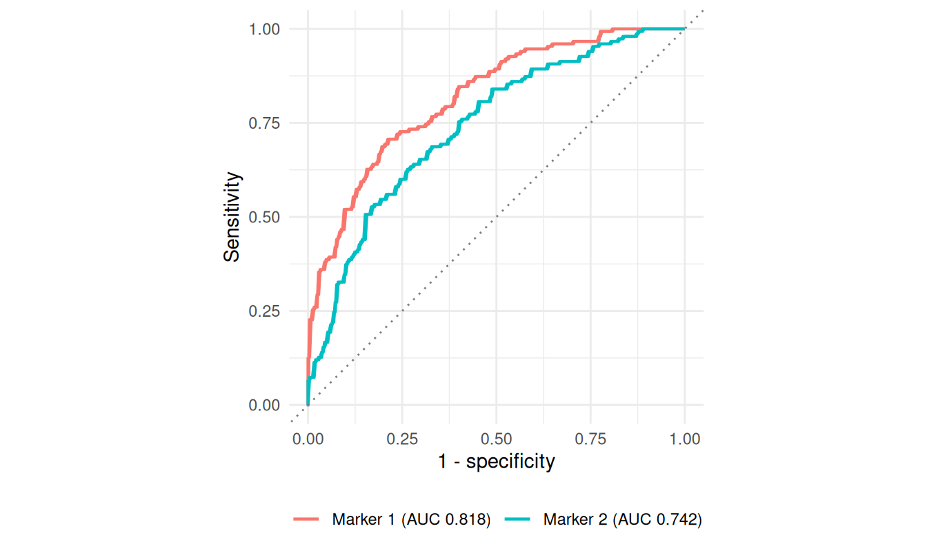
5. Diagnostic accuracy of binary and continuous tests
Tags: [S] primary public source, [Y] my synthesis. All data simulated.
(a) Concept
Measure
Definition
Depends on prevalence?
Sensitivity
P(T+ | D+)
no
Specificity
P(T− | D−)
no
PPV / NPV
P(D+ | T+), P(D− | T−)
yes
LR+ / LR−
Se/(1−Sp), (1−Se)/Sp
no
PPA / NPA / OPA
agreement with a non-reference comparator
–
AUC
P(case marker > control marker)
no
Rule: sensitivity and specificity need a reference standard. Without one, report PPA/NPA. [S: FDA 2007]
(b) Regulatory anchor
Item
Verified fact
Tag
FDA 2007 Statistical Guidance on Reporting Results from Studies Evaluating Diagnostic Tests
Final, issued 13 Mar 2007. “When a new test is evaluated by comparison to a non-reference standard, sensitivity and specificity are not appropriate terms to describe the comparative results.” Estimates are called positive and negative percent agreement. Discrepant resolution discussed as biasing
[S] fda.gov/media/71147
EP12
Ed3, 2023-03-07: binary-output examinations, clinical performance (sens/spec), imprecision near the cut-off (C5/C95), stability, interference
[S] clsi.org
EP24
EP24-A2 (2011, reaffirmed 2016): ROC-based diagnostic accuracy of continuous tests; concepts, not a recipe
se <-0.90; sp <-0.85pv <-t(sapply(c(0.01, 0.05, 0.10, 0.30, 0.50), function(p) predictive_values(se, sp, p)))kable(data.frame(prevalence =c(0.01, 0.05, 0.10, 0.30, 0.50), round(pv, 3)),caption ="Se 0.90, Sp 0.85. Same test, different populations")
Se 0.90, Sp 0.85. Same test, different populations
prevalence
PPV
NPV
LRpos
LRneg
0.01
0.057
0.999
6
0.118
0.05
0.240
0.994
6
0.118
0.10
0.400
0.987
6
0.118
0.30
0.720
0.952
6
0.118
0.50
0.857
0.895
6
0.118
# check Bayes against a simulated population at 10%set.seed(2); N <-2e6; d <-rbinom(N, 1, .10); t <-rbinom(N, 1, ifelse(d ==1, se, 1- sp))c(sim_PPV =sum(t & d) /sum(t), theory =predictive_values(se, sp, .10)[["PPV"]])
  sim_PPV    theory
0.4006862 0.4000000
Paired comparison of two tests on the same patients
Compare sensitivities only within diseased subjects and specificities within non-diseased, using the paired (discordant) counts; an unpaired z-test ignores the correlation. [Y]
Agreement with a non-reference comparator: why PPA ≠ sensitivity
Truth D is hidden. The comparator C itself errs (Se 0.85, Sp 0.99); the candidate T has true Se 0.92, Sp 0.96.
set.seed(53)N <-200000; D <-rbinom(N, 1, .30)C <-rbinom(N, 1, ifelse(D ==1, .85, .01)); T <-rbinom(N, 1, ifelse(D ==1, .92, .04))agr <-report_agreement(T ==1, C ==1)true <-report_2x2(T ==1, D ==1)# discrepant resolution: discordant pairs resolved by the truth, concordant pairs keep the comparator labelresolved <-ifelse(T != C, D, C)dr <-report_2x2(T ==1, resolved ==1)kable(data.frame(Estimate =c("True sensitivity (unknowable)", "True specificity (unknowable)","PPA vs comparator", "NPA vs comparator","'Sensitivity' after discrepant resolution", "'Specificity' after discrepant resolution"),Value =round(c(true$est[1:2], agr$est[1:2], dr$est[1:2]), 4)))
Estimate
Value
True sensitivity (unknowable)
0.9204
True specificity (unknowable)
0.9597
PPA vs comparator
0.8958
NPA vs comparator
0.9062
‘Sensitivity’ after discrepant resolution
0.9312
‘Specificity’ after discrepant resolution
0.9603
PPA/NPA are not estimates of Se/Sp: the comparator’s errors enter. Here PPA (0.896) is below the true Se (0.920) because the comparator’s false positives sit in the denominator; NPA (0.906) is far below the true Sp (0.960) because the comparator’s false negatives make correct candidate positives count as disagreements. The direction depends on the comparator’s error pattern.
Discrepant resolution resolves only the disagreements, so errors made by both tests are never corrected. Here the “sensitivity” rises above the truth (0.931 vs 0.920) while the “specificity” is almost unchanged (0.960 vs 0.960): the bias is real but its size depends on the error structure. FDA 2007 says there is no statistical fix. [S/Y]
Verification bias and the Begg–Greenes correction
Only positives and 20% of negatives are sent to the reference.
set.seed(54)N <-5000; D <-rbinom(N, 1, .30); T <-rbinom(N, 1, ifelse(D ==1, .90, .15))ver <-rbinom(N, 1, ifelse(T ==1, 1, 0.2))naive_se <-sum(T ==1& D ==1& ver ==1) /sum(D ==1& ver ==1)naive_sp <-sum(T ==0& D ==0& ver ==1) /sum(D ==0& ver ==1)# Begg-Greenes: P(D|T) from verified, P(T) from everyonepDpos <-mean(D[T ==1& ver ==1]); pDneg <-mean(D[T ==0& ver ==1]); pT <-mean(T)bg_se <- pDpos * pT / (pDpos * pT + pDneg * (1- pT))bg_sp <- (1- pDneg) * (1- pT) / ((1- pDneg) * (1- pT) + (1- pDpos) * pT)kable(data.frame(estimate =c("Complete-data truth", "Naive (verified only)", "Begg-Greenes corrected"),Sensitivity =round(c(sum(T & D) /sum(D), naive_se, bg_se), 3),Specificity =round(c(sum(!T &!D) /sum(!D), naive_sp, bg_sp), 3)))
estimate
Sensitivity
Specificity
Complete-data truth
0.901
0.834
Naive (verified only)
0.979
0.508
Begg-Greenes corrected
0.907
0.835
Naive sensitivity is inflated, specificity deflated. Correction assumes verification depends only on the test result. [Y]
stopifnot(abs(as.numeric(pa) - pa_hand) <0.003) # differ in the 3rd decimal: interpolation at the 0.90 boundary
(d) Claims
FDA 2007 guidance statements, EP12/EP24 editions, STARD 2015 and QUADAS-2 citations, IVDR Annex I 9.1(b) are in the ledger (chapters 1/5). Everything tagged [Y] is theory, not quoted.