Tags: [S] primary public source, [Y] my synthesis, [A] assumption. Every number below is computed two ways (package vs hand, or hand vs simulation).
(a) Concept
Goal
Quantity to fix
Typical output
Estimate Se or Sp precisely
CI half-width d, expected Se/Sp, prevalence
n cases, then total n = cases / prevalence
Show Se (or Sp) exceeds a performance goal
goal p0, expected p1, α, power
n cases (exact binomial)
Show AUC > AUC0 or estimate AUC precisely
expected AUC, null, group ratio
n cases and controls
PPA/NPA vs a comparator
as Se/Sp but denominators are comparator-positive/negative
total n via comparator prevalence
Precision studies
days, runs, replicates
degrees of freedom → CI width
LoB/LoD
number of blanks and low samples
precision of the percentile / SD
Total n is driven by the rarest class: for sensitivity you need cases, and cases arrive at the rate of the prevalence. [Y]
(b) Anchor
Item
Verified fact
Tag
Buderer 1996
“Statistical methodology: I. Incorporating the prevalence of disease into the sample size calculation for sensitivity and specificity.” Acad Emerg Med 3(9):895-900. Sample size from desired precision, hypothesised Se/Sp and prevalence
[S] abstract
Flahault et al. 2005
J Clin Epidemiol 58(8):859-862. Case numbers for expected sensitivity 0.60-0.99 and acceptable lower 95% limit 0.50-0.98, with 5% probability the estimated lower limit falls below the acceptable level
[S] abstract; tables not opened
Hanley & McNeil 1982
Radiology 143(1):29-36. SE formulas for AUC; AUC = P(case > control)
[S] abstract
Obuchowski
AJR 2000;175:603-8 “Sample size tables for ROC studies” (multi-observer imaging). The 1994 Invest Radiol paper is also a candidate; the commonly cited reference is ambiguous
[S] metadata
IVDR Annex XIII Part A 2.3.2
The clinical performance study plan must justify statistical design and population size (items (j), (m))
[S]
Design counts in EP05/EP17 (days, blanks)
Public: EP05-A3 20×2×2. EP17 counts not verified: paywalled
–
(c) R lab
1. Estimate Se/Sp to a target half-width
Expected Se = 0.90, half-width ±0.05, prevalence 0.20.
d <-0.05; se <-0.90; prev <-0.20hand_wald <-n_buderer(se, d, prev) # Buderer, normal approximationpz <-prec_sens(se, prev = prev, conf.width =2* d) # Wilson-based (presize)cases_wald <-ceiling(qnorm(.975)^2* se * (1- se) / d^2)kable(data.frame(Method =c("Buderer / Wald (hand)", "presize Wilson"),`Cases`=c(cases_wald, ceiling(pz$n)),`Total n at prevalence 0.20`=c(hand_wald, ceiling(pz$ntot)),check.names =FALSE))
Method
Cases
Total n at prevalence 0.20
Buderer / Wald (hand)
139
692
presize Wilson
141
705
# simulation: achieved Wilson half-width at n = 141 casesset.seed(71)hw <-replicate(5000, { x <-rbinom(1, 141, se); w <-ci_wilson(x, 141); (w[["upper"]] - w[["lower"]]) /2 })c(sim_mean_halfwidth =mean(hw))
sim_mean_halfwidth
        0.04964971
Wald slightly under-sizes relative to Wilson at p = 0.9 (139 vs 141 cases); the simulation confirms the Wilson design reaches ±0.05. [Y]
2. Prevalence inflates the total n
pv <-c(0.01, 0.05, 0.10, 0.20, 0.40)kable(data.frame(Prevalence = pv,`Total n for Se +-0.05`=sapply(pv, function(p) ceiling(prec_sens(0.9, prev = p, conf.width =0.1)$ntot)),`Total n for Sp +-0.05`=sapply(pv, function(p) ceiling(prec_spec(0.9, prev = p, conf.width =0.1)$ntot)),check.names =FALSE), caption ="Se = Sp = 0.90. Rare condition: huge n for sensitivity")
Se = Sp = 0.90. Rare condition: huge n for sensitivity
Prevalence
Total n for Se +-0.05
Total n for Sp +-0.05
0.01
14098
143
0.05
2820
149
0.10
1410
157
0.20
705
177
0.40
353
235
When prevalence is low, enrich (case-control or stratified sampling) and state the consequence: PPV/NPV cannot be read from an enriched sample without reweighting. [Y]
3. Show sensitivity beats a performance goal (exact test)
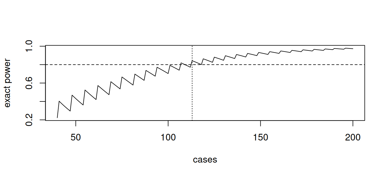
Expected Se p1 = 0.90, goal p0 = 0.80, one-sided α = 0.025 (matches a two-sided 95% CI), power 80%.
n_hand <-n_exact_goal_stable(0.90, 0.80, alpha =0.025, power =0.80)n_mk <-power.diagnostic.test(sens =0.9, delta =0.1, power =0.8, sig.level =0.025, prev =0.2)$n# simulation: power at n_hand with exact one-sided binom.testset.seed(72)pw <-mean(replicate(4000, binom.test(rbinom(1, n_hand, .9), n_hand, p = .8, alternative ="greater")$p.value < .025))# closed-form normal approximationza <-qnorm(.975); zb <-qnorm(.80)n_norm <-ceiling(((za *sqrt(.8* .2) + zb *sqrt(.9* .1)) / (.9- .8))^2)kable(data.frame(Method =c("exact, hand (stable)", "MKmisc::power.diagnostic.test", "normal approximation", "simulated power at n(hand)"),Value =c(n_hand, n_mk, n_norm, round(pw, 3))))
Method
Value
exact, hand (stable)
113.000
MKmisc::power.diagnostic.test
113.000
normal approximation
108.000
simulated power at n(hand)
0.843
stopifnot(n_hand == n_mk)
Exact power is a sawtooth in n (discreteness); report the smallest n above which power never falls below target. Total n = cases / prevalence. [Y] My reading of Flahault 2005 is the same type of calculation (expected Se vs an acceptable lower limit); its tables were not opened.
Expected AUC 0.90; test against AUC0 = 0.75, two-sided α = 0.05, 80% power, 1:1 cases:controls.
n_h <-n_auc_hm(0.90, 0.75, alpha =0.05, power =0.80)# simulation with the binormal model: AUC = pnorm(delta/sqrt(2)) for equal unit variancesdelta <-function(a) sqrt(2) *qnorm(a)set.seed(73)sim_power <-function(n, a1 =0.90, a0 =0.75, reps =600) {mean(replicate(reps, { cs <-rnorm(n, delta(a1)); ct <-rnorm(n) r <-roc(rep(1:0, each = n), c(cs, ct), quiet =TRUE, direction ="<") ci <-ci.auc(r, method ="delong") # reject if the lower 95% limit exceeds AUC0 (as.numeric(ci)[1] > a0) }))}grid <-c(20, 24, 28, n_h)kable(data.frame(`Cases = controls`= grid, `Simulated power`=sapply(grid, sim_power),check.names =FALSE),caption =sprintf("Hanley-McNeil n = %d per group; power by simulation (600 reps)", n_h))
Hanley-McNeil n = 34 per group; power by simulation (600 reps)
Cases = controls
Simulated power
20
0.7800000
24
0.8550000
28
0.8766667
34
0.9266667
The Hanley–McNeil formula is conservative here: the simulated power at its n is well above 80%, and 80% is reached with fewer subjects. The simulated rule (DeLong lower 95% limit > AUC0) is a one-sided α = 0.025 test, which is the same critical value as the two-sided 0.05 used in the formula, so the gap comes from the variance approximation, not the α. Use the formula to plan, simulation to confirm. [Y]
Cross-check against pROC::power.roc.test (which handles AUC vs 0.5 only) and presize (CI half-width):
n_h5 <-n_auc_hm(0.75, 0.5, alpha =0.05, power =0.80)pr <-power.roc.test(auc =0.75, sig.level =0.05, power =0.80)kable(data.frame(Check =c("HM hand, AUC 0.75 vs 0.5", "pROC::power.roc.test, same"),`Cases (= controls)`=c(n_h5, ceiling(pr$ncases)), check.names =FALSE))
Check
Cases (= controls)
HM hand, AUC 0.75 vs 0.5
20
pROC::power.roc.test, same
19
# precision: n for 95% CI width 0.10 at AUC 0.90, prevalence 0.4pa <-prec_auc(0.9, prev =0.4, conf.width =0.10)hm_hw <-function(n1) 1.96*sqrt(var_auc_hm(0.9, n1, 1.5* n1))n1_hand <-ceiling(uniroot(function(n1) hm_hw(n1) -0.05, c(10, 2000))$root)c(presize_cases =ceiling(pa$n1), HM_hand_cases = n1_hand)
presize_cases HM_hand_cases
           75            75
5. PPA/NPA and the indeterminate fraction
When intermediates count as non-agreement, the quantity to size is PPA_incl = Se_det·(1 − f_D) where f_D is the intermediate fraction among comparator-positives.
Two decisions to pre-specify: the endpoint including vs excluding indeterminates, and the sample size to secure enough determinate results (divide by 1 − f). [Y]
6. Design sizes for EP05 and EP17-type studies (illustrative)
Precision, CI width of within-lab SD versus number of days. Satterthwaite df of the sum of mean squares; hand check against VCA’s DF for the Chapter 2 data.
sat_df <-function(ms, D, R, K) { cf <-c(day =1/ (R * K), run = (R -1) / (R * K), err = (K -1) / K) df <-c(D -1, D * (R -1), D * R * (K -1))sum(cf * ms)^2/sum((cf * ms)^2/ df)}# MS from the Chapter 2 simulated study (VCA output): day 9.906929, run 5.628042, error 4.808839df_hand <-sat_df(c(9.906929, 5.628042, 4.808839), 20, 2, 2)c(hand = df_hand, VCA_reported =69.815065)
        hand VCA_reported
    69.81506     69.81507
stopifnot(abs(df_hand -69.815065) <1e-3)ci_ratio <-function(D, R =2, K =2, sd_d =1.2, sd_r =1.5, sd_e =2) { ms <-c(sd_e^2+ K * sd_r^2+ R * K * sd_d^2, sd_e^2+ K * sd_r^2, sd_e^2) df <-sat_df(ms, D, R, K)c(days = D, df = df, `upper/estimate`=sqrt(df /qchisq(.025, df)), `lower/estimate`=sqrt(df /qchisq(.975, df)))}kable(t(sapply(c(5, 10, 20, 30, 40), ci_ratio)), digits =3,caption ="Expected 95% CI of within-lab SD as multiples of the estimate (2 runs x 2 replicates)")
Expected 95% CI of within-lab SD as multiples of the estimate (2 runs x 2 replicates)
days
df
upper/estimate
lower/estimate
5
13.199
1.604
0.726
10
28.655
1.347
0.795
20
59.452
1.219
0.848
30
90.224
1.171
0.873
40
120.990
1.144
0.888
LoB: precision of the 95th percentile vs number of blanks.
set.seed(74)sim_lob <-function(n, B =4000) { p <-replicate(B, { b <-rnorm(n); c(np =unname(quantile(b, .95, type =6)), par =mean(b) +1.645*sd(b)) })data.frame(blanks = n, `SD nonparametric`=sd(p["np", ]), `SD parametric`=sd(p["par", ]),`theory SD parametric`=sqrt(1/ n +1.645^2/ (2* (n -1))), check.names =FALSE)}kable(do.call(rbind, lapply(c(20, 60, 120, 240), sim_lob)), digits =3,caption ="Blank ~ N(0,1): SD of the LoB estimate (units of the blank SD)")
Blank ~ N(0,1): SD of the LoB estimate (units of the blank SD)
blanks
SD nonparametric
SD parametric
theory SD parametric
20
0.514
0.344
0.348
60
0.280
0.199
0.199
120
0.197
0.143
0.140
240
0.136
0.099
0.099
The parametric estimator is more precise (it uses all data and the normal assumption); the closed form sqrt(1/n + 1.645²/(2(n−1))) agrees with the simulation. [Y]
(d) Claims
Buderer, Flahault, Hanley–McNeil, Obuchowski metadata and the ambiguity of the Obuchowski reference are in the ledger.