set.seed(11)
n <- 100
t <- exp(runif(n, log(5), log(500)))
x <- t * (1 + rnorm(n, 0, 0.03))
y <- 2 + 1.06 * t * (1 + rnorm(n, 0, 0.04))
y[c(10, 50, 90)] <- y[c(10, 50, 90)] * c(1.5, 0.6, 1.7)   # outliers
dat <- data.frame(x, y)4. Method comparison, bias, interference, stability, lots
Tags: [S] primary public source, [Y] my synthesis. All data simulated.
(a) Concept
| Study | Question | Core statistic |
|---|---|---|
| Method comparison (EP09c) | Do candidate and comparator agree? Bias at decision levels? | Deming / Passing–Bablok regression, bias with CI |
| Interference (EP07) | Does a substance change the result by more than allowable error? | paired difference ± CI vs allowable limit |
| Reagent stability (EP25) | How long until results drift beyond a limit? | regression over time, bound crossing the limit |
| Lot-to-lot (EP26) | Does a new lot shift patient results by a clinically important amount? | paired difference ± CI vs acceptable difference |
OLS assumes x is error-free. Both methods have error, so use errors-in-variables regression: Deming (normal errors, outlier-sensitive) or Passing–Bablok (rank-based, robust, needs a roughly linear relation). [Y]
(b) Regulatory anchor
| Document | Verified fact | Tag |
|---|---|---|
| EP09c | Ed3 corrected, 2018-06-20; EP09-A3 (2013) withdrawn 2018. Design/analysis of method comparison with patient samples to estimate bias | [S] clsi.org |
| EP07 | Ed3, 2018-04-30, confirmed 2022; screening, quantifying, confirming interference; EP37 = supplemental interferent-concentration tables (edition not verified) | [S] clsi.org |
| EP25 | Ed2, 2023-04-26 (replaces EP25-A, 2009); regression-based shelf-life and in-use stability | [S] clsi.org |
| EP26 | Ed2, 2022-04-27 (replaces EP26-A, 2013); user evaluation of reagent lot change with a small number of patient samples | [S] clsi.org |
| Sample counts, concentration-range rules, allowable-error rules | not verified: paywalled (the often-quoted ≥ 100 samples for EP09 is therefore not asserted) | – |
| IVDR | Annex I 9.1(a): trueness (bias), precision, interference-related analytical specificity | [S] |
(c) R lab
Simulated comparison
True concentrations 5–500 (log-uniform), reference method CV 3%, candidate has +2 constant and +6% proportional bias, CV 4%, plus 3 gross outliers.
OLS, Deming, Passing–Bablok
fit_ols <- lm(y ~ x)
fit_dem <- mcreg(x, y, method.reg = "WDeming", error.ratio = 1, method.ci = "jackknife")
Jackknife based calculation of standard error and confidence intervals according to Linnet's method.fit_pb <- mcreg(x, y, method.reg = "PaBa", method.ci = "bootstrap", method.bootstrap.ci = "BCa", nsamples = 999)
ci_ols <- confint(fit_ols)
tab <- rbind(
data.frame(Method = "OLS", Intercept = coef(fit_ols)[1], Slope = coef(fit_ols)[2],
`Int 95% CI` = sprintf("%.2f to %.2f", ci_ols[1, 1], ci_ols[1, 2]),
`Slope 95% CI` = sprintf("%.3f to %.3f", ci_ols[2, 1], ci_ols[2, 2])),
data.frame(Method = "Weighted Deming", Intercept = fit_dem@para[1, 1], Slope = fit_dem@para[2, 1],
`Int 95% CI` = sprintf("%.2f to %.2f", fit_dem@para[1, 3], fit_dem@para[1, 4]),
`Slope 95% CI` = sprintf("%.3f to %.3f", fit_dem@para[2, 3], fit_dem@para[2, 4])),
data.frame(Method = "Passing-Bablok", Intercept = fit_pb@para[1, 1], Slope = fit_pb@para[2, 1],
`Int 95% CI` = sprintf("%.2f to %.2f", fit_pb@para[1, 3], fit_pb@para[1, 4]),
`Slope 95% CI` = sprintf("%.3f to %.3f", fit_pb@para[2, 3], fit_pb@para[2, 4])))
names(tab) <- c("Method", "Intercept", "Slope", "Int 95% CI", "Slope 95% CI")
kable(tab, digits = 3, row.names = FALSE,
caption = "True intercept 2, slope 1.06; 3 outliers present")| Method | Intercept | Slope | Int 95% CI | Slope 95% CI |
|---|---|---|---|---|
| OLS | 2.491 | 1.046 | -0.24 to 5.22 | 1.021 to 1.071 |
| Weighted Deming | 2.238 | 1.055 | 1.91 to 2.56 | 1.027 to 1.082 |
| Passing-Bablok | 2.027 | 1.064 | 1.73 to 2.36 | 1.035 to 1.081 |
Cross-check of point estimates against hand implementations (rule 4):
dem_pkg <- mcreg(x, y, method.reg = "Deming", error.ratio = 1, method.ci = "analytical")@para[, 1]
pb_pkg  <- mcreg(x, y, method.reg = "PaBa", method.ci = "analytical")@para[, 1]
chk <- data.frame(
  estimate = c("Deming intercept", "Deming slope", "PaBa intercept", "PaBa slope"),
  package = c(dem_pkg, pb_pkg), hand = c(deming_hand(x, y, 1), paba_hand(x, y)))
kable(chk, digits = 5)| estimate | package | hand |
|---|---|---|
| Deming intercept | 1.96850 | 1.96850 |
| Deming slope | 1.05405 | 1.05405 |
| PaBa intercept | 2.02662 | 2.02662 |
| PaBa slope | 1.06388 | 1.06388 |
stopifnot(isTRUE(all.equal(chk$package, chk$hand, tolerance = 1e-6)))ggplot(dat, aes(x, y)) + geom_point(alpha = .6) +
geom_abline(slope = 1, intercept = 0, colour = "grey50", linetype = 3) +
geom_abline(slope = coef(fit_ols)[2], intercept = coef(fit_ols)[1], colour = "#1b9e77") +
geom_abline(slope = fit_dem@para[2, 1], intercept = fit_dem@para[1, 1], colour = "#7570b3") +
geom_abline(slope = fit_pb@para[2, 1], intercept = fit_pb@para[1, 1], colour = "#d95f02") +
scale_x_log10() + scale_y_log10() +
labs(x = "Comparator", y = "Candidate",
subtitle = "dotted = identity; green OLS, purple Deming, orange Passing-Bablok") +
theme_minimal()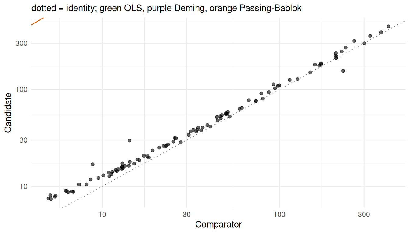
OLS is pulled by the outliers and by errors in x; Passing–Bablok stays near the truth. [Y]
Bias at medical decision levels
lv <- c(20, 100, 300)
bd <- as.data.frame(calcBias(fit_dem, x.levels = lv))
bp <- as.data.frame(calcBias(fit_pb,  x.levels = lv))
hand_bias <- function(p, l) p[1] + (p[2] - 1) * l      # a + (b-1)*Xc
kable(data.frame(
  `Decision level` = lv,
  `Deming bias (95% CI)` = sprintf("%.2f (%.2f to %.2f)", bd$Bias, bd$LCI, bd$UCI),
  `PaBa bias (95% CI)` = sprintf("%.2f (%.2f to %.2f)", bp$Bias, bp$LCI, bp$UCI),
  `Hand a+(b-1)Xc, PaBa` = round(hand_bias(fit_pb@para[, 1], lv), 2),
  `Rel. bias % (PaBa)` = round(100 * bp$Bias / lv, 1), check.names = FALSE),
caption = "Bias at decision levels; true bias = 2 + 0.06 X")| Decision level | Deming bias (95% CI) | PaBa bias (95% CI) | Hand a+(b-1)Xc, PaBa | Rel. bias % (PaBa) |
|---|---|---|---|---|
| 20 | 3.33 (2.91 to 3.75) | 3.30 (3.09 to 3.61) | 3.30 | 16.5 |
| 100 | 7.71 (5.15 to 10.27) | 8.42 (5.78 to 9.93) | 8.42 | 8.4 |
| 300 | 18.66 (10.58 to 26.73) | 21.19 (12.75 to 26.08) | 21.19 | 7.1 |
stopifnot(isTRUE(all.equal(bp$Bias, hand_bias(fit_pb@para[, 1], lv), tolerance = 1e-8)))Bland–Altman with proportional bias
ba <- data.frame(mean = (x + y) / 2, rel = 100 * (y - x) / ((x + y) / 2))
pbias <- lm(rel ~ log10(mean), ba)
loa <- mean(ba$rel) + c(-1.96, 1.96) * sd(ba$rel)
ggplot(ba, aes(mean, rel)) + geom_point(alpha = .6) + scale_x_log10() +
  geom_hline(yintercept = c(mean(ba$rel), loa), linetype = c(1, 2, 2)) +
  geom_smooth(method = "lm", se = FALSE, colour = "#d95f02") +
  labs(x = "Mean of the two methods", y = "Difference (%)") + theme_minimal()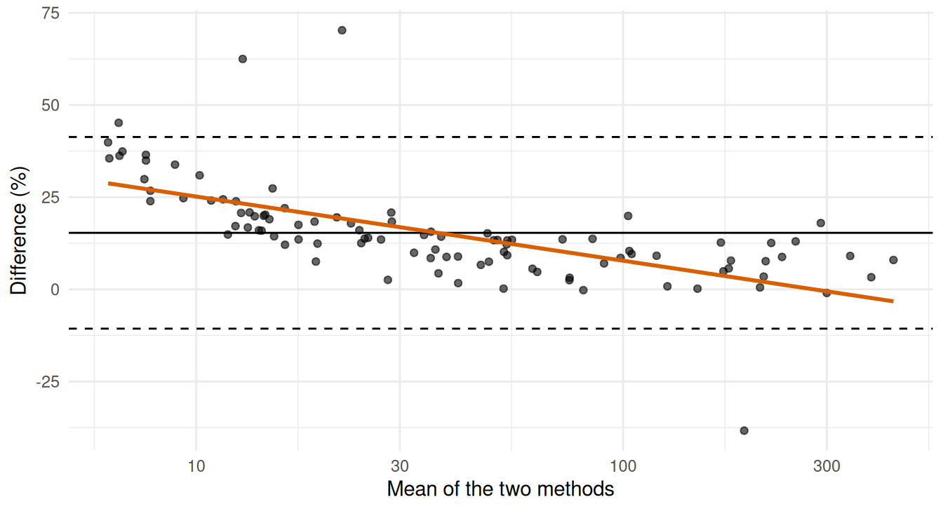
c(mean_diff_pct = mean(ba$rel), LoA_lo = loa[1], LoA_hi = loa[2],
  p_trend = summary(pbias)$coefficients[2, 4])
mean_diff_pct LoA_lo LoA_hi p_trend
1.533644e+01 -1.065647e+01 4.132935e+01 3.347871e-13 A significant trend of relative difference with level signals bias that depends on concentration (here the constant +2 matters at low levels). Limits of agreement do not replace a regression-based bias estimate at decision levels. [Y]
Interference (EP07 logic) [Y]
set.seed(70)
ctrl <- rnorm(10, 100, 3); test <- rnorm(10, 104, 3)            # true +4% effect
d <- test - ctrl; se <- sd(d) / sqrt(10)
ci <- mean(d) + c(-1, 1) * qt(.975, 9) * se
tt <- t.test(test, ctrl, paired = TRUE)
allow <- 10                                                  # assumed allowable error, % of 100
data.frame(mean_diff = mean(d), lo = ci[1], hi = ci[2], t_test_lo = tt$conf.int[1],
           t_test_hi = tt$conf.int[2], within_allowable = all(abs(ci) <= allow))
mean_diff lo hi t_test_lo t_test_hi within_allowable
1 6.201981 4.358726 8.045237 4.358726 8.045237 TRUEstopifnot(isTRUE(all.equal(ci, as.numeric(tt$conf.int))))Conclude “no clinically relevant interference” only if the whole CI sits inside the allowable limit, not because the test is non-significant. [Y]
Reagent stability (EP25 logic) [Y]
set.seed(25)
mo <- rep(c(0, 2, 4, 6, 8, 10, 12), each = 3)
val <- 100 - 0.45 * mo + rnorm(length(mo), 0, 0.8)
fit <- lm(val ~ mo)
grid <- data.frame(mo = seq(0, 24, 0.1))
pr <- predict(fit, grid, se.fit = TRUE)
lower <- pr$fit - qt(.95, df.residual(fit)) * pr$se.fit       # one-sided 95% lower bound
limit <- 95
shelf <- grid$mo[which(lower < limit)[1]]
shelf_hand <- {
  f <- function(t) { s <- summary(fit); xb <- mean(mo); sxx <- sum((mo - xb)^2)
    se <- s$sigma * sqrt(1 / length(mo) + (t - xb)^2 / sxx)
    coef(fit)[1] + coef(fit)[2] * t - qt(.95, df.residual(fit)) * se - limit }
  uniroot(f, c(0, 24))$root }
c(shelf_life_months = shelf, hand_uniroot = shelf_hand)
shelf_life_months hand_uniroot
10.30000 10.28842 stopifnot(abs(shelf - shelf_hand) < 0.1)Claim the shelf life at the time the one-sided bound crosses the acceptance limit (here a 5% loss), not where the mean line does. EP25 Ed2’s exact acceptance rules: not verified: paywalled.
Lot-to-lot (EP26 logic) [Y]
set.seed(26)
m <- 40
base <- exp(runif(m, log(10), log(400)))
lotA <- base * (1 + rnorm(m, 0, .02)); lotB <- base * 1.015 * (1 + rnorm(m, 0, .02))
pd <- 100 * (lotB - lotA) / lotA
ci <- mean(pd) + c(-1, 1) * qt(.975, m - 1) * sd(pd) / sqrt(m)
mad <- 3                                                   # assumed medically acceptable difference, %
data.frame(mean_pct_diff = mean(pd), lo = ci[1], hi = ci[2],
           acceptable = ci[2] < mad & ci[1] > -mad)
mean_pct_diff lo hi acceptable
1 1.196325 0.2454338 2.147216 TRUE(d) Claims
Editions and scopes for EP09c, EP07, EP37, EP25, EP26 are in the ledger. Design counts and acceptance criteria: not verified: paywalled.